How quickly does digital level measurement for IBCs pay for itself?
The honest answer is: It doesn't depend solely on the technology used. What matters most is how the new data changes day-to-day operations.
Are reorders triggered sooner? Are safety stock levels decreasing? Are IBCs being turned over more quickly? Are fewer new containers needed? Are there fewer express deliveries? And how much time do employees currently spend searching for containers, checking fill levels, and reconciling Excel spreadsheets?
This is precisely where the economic value of IBC digitization lies.
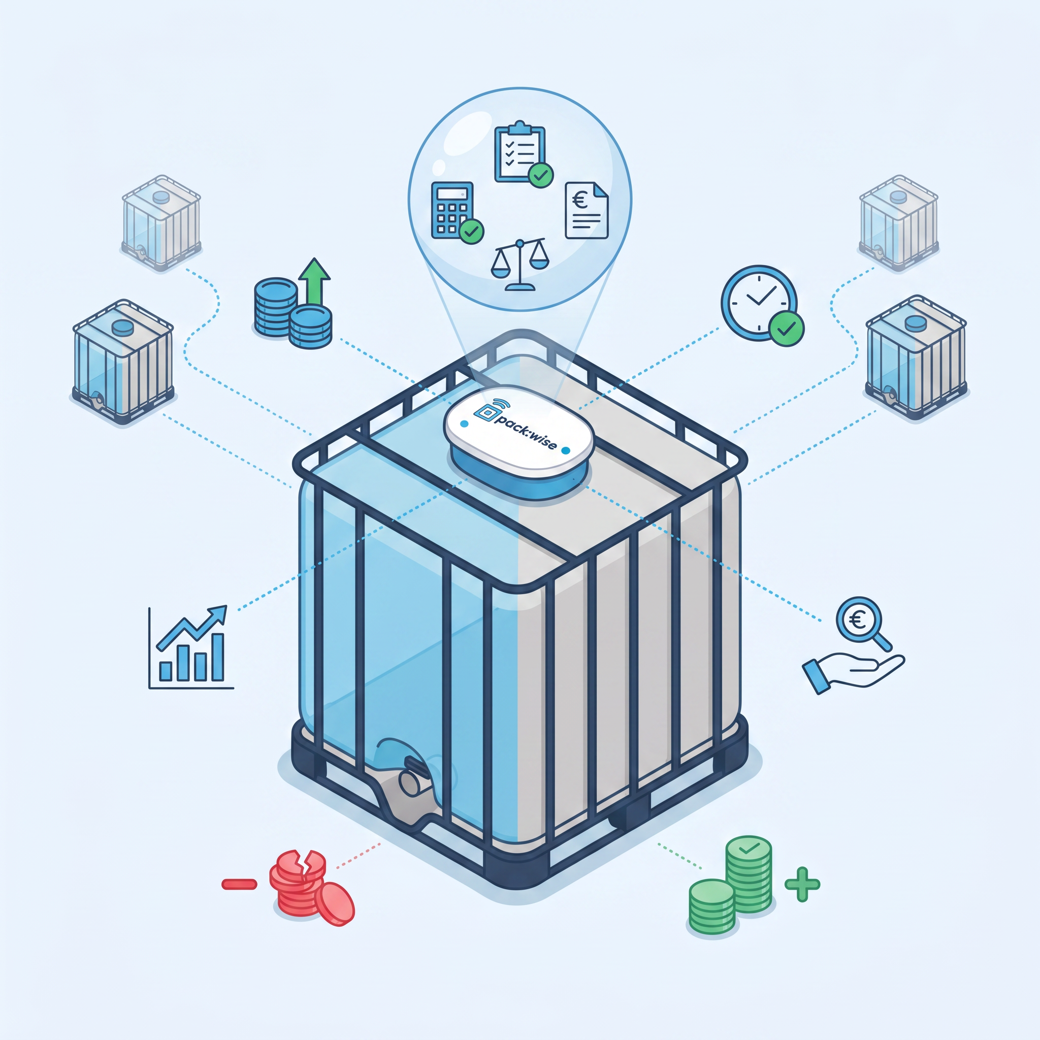
The Packwise Smart Cap collects data on fill level, temperature, location, and movement directly from the container. Packwise Flow makes this information available, can integrate it into existing systems, and can trigger notifications or follow-up processes when specific events occur. This transforms an analog IBC into a digital data source for inventory management, logistics, and supply chain control.
In this article, we'll walk through the ROI step by step—without financial acrobatics, without a hardware price list, and without hidden calculation assumptions.
To do this, we'll use two models:
- a quick ROI check for a pilot project with 80 digitized IBCs,
- a detailed fleet business case for 350 IBCs.
All parameters, formulas, and assumptions are fully disclosed.
Important note: All euro amounts in the two calculation examples are fictitious model assumptions. They are neither a Packwise price list nor a specific offer nor a general guarantee of success. The actual costs and potential depend on the specific fleet, processes, container types, locations, integrations, and objectives.
The more important question: What does it cost not to digitize?
The costs of digitization are generally transparent. There are one-time project costs, ongoing operating costs, and internal effort for implementation and process adaptation.
The costs of a non-digitized IBC fleet are much better hidden.
They are spread out, for example, across:
- excessive safety stock,
- tied-up product capital,
- an unnecessary number of IBCs,
- lost or untraceable containers,
- long dwell times at the customer's site,
- manual reconciliation,
- unplanned express deliveries,
- delayed reorders,
- production interruptions and stockouts.
None of these items are listed in accounting as "missing inventory data." Together, however, they can have a significant economic impact.
For existing reusable container fleets, Packwise cites, among other things, reduced manual tracking effort, a lower loss rate, higher fleet utilization, and lower costs for new container purchases as relevant areas of application. Turnover and downtime can be evaluated as supply chain KPIs.
No hardware unit prices—but a complete cost calculation nonetheless
To calculate ROI, there is no need to publicly disclose hardware prices per device.
Mathematically, it is sufficient to work with two complete cost categories:
One-time project costs
These may include technical deployment, configuration, implementation, commissioning, integration, training, and rollout. A total amount is used for these in the business case.
Ongoing project costs
These may include platform usage, connectivity, data processing, support, and other ongoing services. Here, too, a total amount per month or year is sufficient.
Breaking down a proposal into individual technical components is not required for the ROI formula.
The only important thing is that all costs are taken into account and no item is omitted without being noticed.
ROI, payback, and capital release are not the same thing
In ROI calculations, various effects are often combined into a single large number. This sounds impressive, but it is of little help in making a sound investment decision.
A clear distinction is better.
| Key metric |
What it answers |
| Annual gross savings |
What operational value does digitization generate before ongoing project costs? |
| Annual net benefit |
What remains after deducting ongoing project costs? |
| ROI |
How high is the economic surplus relative to the total costs? |
| Payback |
How long does it take to recoup the initial investment? |
| One-time capital impact |
What investments are avoided, or what working capital is freed up? |
The classic ROI formula is:
ROI = (Total Benefits − Total Costs) ÷ Total Costs × 100
For a simple payback calculation:
Payback = one-time project costs ÷ monthly net benefit
The monthly net benefit is calculated as follows:
Monthly net benefit = monthly gross savings − ongoing project costs
If the implementation or ramp-up period is longer, this must also be taken into account.
What data do you need for a reliable IBC ROI?
Don't worry: You don't need a months-long controlling project to make an initial calculation.
Much of the information is already available in Purchasing, Logistics, Finance, Customer Service, or Supply Chain Management.
Data on the container fleet
The following are particularly relevant:
- current fleet size,
- value or replacement cost of an IBC,
- number of cycles per year,
- average turnaround time,
- safety stock,
- Loss rate,
- Inspection and maintenance intervals.
Product inventory data
For example, the following are required:
- Volume of an IBC,
- average product value per liter,
- Lifespan of full or partially filled IBCs at the customer's site,
- expected reduction in dwell time,
- the company's cost of capital.
Data on operational processes
This includes:
- Time spent on searching and coordination,
- Full costs of the employees involved,
- Number of unplanned express deliveries,
- Additional costs per express delivery,
- complaints and special processes,
- Costs of potential stockouts or production stoppages.
Project Data
The following are required for the investment side:
- total one-time project costs,
- ongoing project costs,
- internal implementation costs,
- expected ramp-up,
- the analysis period.
This establishes the basic framework.
The Key Value Drivers of IBC Digitization
Not every IBC fleet generates its highest ROI in the same area. For one company, express deliveries may be the dominant factor; for another, it might be capital tied up or the number of lost containers.
The following value drivers therefore form a modular framework. A specific business case should include only those effects that are actually relevant and can be plausibly demonstrated.
1. More cycles can reduce fleet requirements
An IBC that remains unnecessarily long at a customer's site, in an intermediate warehouse, or at an unknown location is missing from elsewhere in the cycle.
The company often responds to this by adding more containers and maintaining a larger safety stock.
If the location, fill level, and dwell times are visible, retrieval, refilling, and replenishment can be managed more precisely. As a result, the same delivery volume can potentially be moved using fewer containers.
A simplified calculation is:
Operational IBCs today = current fleet × (1 − current safety stock)
Operational IBCs at target = operational IBCs today × current turnover ÷ target turnover
Target fleet = operational IBCs at target + target safety stock
Reduced fleet requirement = current fleet − target fleet
The economic value then arises on two levels:
- as avoided or freed-up investment in IBCs,
- as annual savings in capital costs.
2. Less tied-up product capital
A full IBC contains not only material but also capital.
With a volume of 1,000 liters and a product value of two euros per liter, a full IBC contains goods worth 2,000 euros.
If many full or barely used containers remain at the customer's site for a long time, a correspondingly large amount of working capital is tied up outside the company's own facility.
The product value per IBC is calculated as follows:
Product value per IBC = IBC volume × product value per liter
The length of an average cycle is calculated as follows:
Cycle duration in days = 365 ÷ number of cycles per year
The proportion of the cycle duration that an IBC spends full at the customer's site can then be determined.
Product capital at the customer's site = product value per IBC × operational IBCs × time spent at the customer's site ÷ cycle duration
If the dwell time is reduced, the average product inventory in the field decreases.
An important distinction must be made here:
Released product capital is a one-time working capital effect.
Capital cost savings represent the resulting annual economic benefit.
3. Lower capital costs for the IBC fleet
If a company requires fewer IBCs in the future, correspondingly less capital will be tied up in containers.
For example, if 100 IBCs are avoided and each container is worth 2,500 euros, the capital effect amounts to 250,000 euros.
At a cost of capital of ten percent, this results in:
€250,000 × 10% = €25,000 in annual capital cost savings
Whether this value is classified internally as financing costs, opportunity costs, or a reduction in capital employed should be determined in consultation with the Finance department.
4. Fewer Lost Containers
Without end-to-end transparency, IBCs can be left at customer sites, misallocated, or disappear entirely from the cycle.
The current annual loss costs can be easily calculated:
Annual loss costs = Fleet size × Loss rate × IBC value
For a realistic business case, a loss prevention rate should then be applied:
Avoidable loss = annual loss costs × avoidable percentage
A prevention rate of 100 percent is an ambitious model assumption. For conservative calculations, rates of 50, 60, or 80 percent can be used, for example.
5. Fewer Inspection and Maintenance Events
A smaller fleet results in fewer inspections, inner tank replacements, and maintenance events.
Assuming an inspection every 2.5 years:
Annual inspection costs = fleet size ÷ 2.5 × cost per inspection
The savings result from the difference between the current fleet and the fleet that will be needed in the future.
The same applies to other periodic replacement or maintenance events.
6. Less manual effort
Container management is often not a single, clearly defined job role.
The workload is distributed across scheduling, logistics, sales, customer service, purchasing, and accounting.
Typical tasks include:
- searching for missing IBCs,
- checking fill levels by phone or email,
- updating lists,
- coordinating returns,
- reconciling ERP data with physical inventory,
- Remind customers to place reorders.
The economic value of automation can be calculated as the capacity freed up:
Capacity value = FTEs involved × full cost per FTE × reducible share of work
A calculated savings of 0.5 FTE does not automatically mean that half a position is eliminated.
It can also mean that existing employees can serve more customers, work fewer overtime hours, respond more quickly, or focus on higher-value tasks.
7. Fewer Express Deliveries and Stockouts
If low inventory is not detected until the customer calls, the only option is often an unplanned express delivery.
With continuous inventory data, restocking can be planned earlier. Packwise Flow, for example, can trigger notifications when material levels are low and support follow-up processes such as reorders or pickups. (Packwise)
The calculation is as follows:
Current express shipping costs = number of express deliveries per year × additional cost per express delivery
Savings = current express costs × expected reduction
Potential follow-up costs of a stockout—such as production interruptions or impacts on customer relationships—are not automatically included. Such effects should only be monetized if reliable data is available.
Model Calculation 1: The Quick ROI Check for 80 Digitized IBCs
The first calculation is suitable for early budget discussions or a pilot project.
The benefit is not yet derived from each individual process formula. Instead, a monthly economic benefit per digitized IBC is assumed.
This is quick and easy to understand. However, the input values should be replaced later with actual pilot data.
All parameters of the model calculation
| Parameters |
Model Assumption |
| Number of digitized IBCs |
80 |
| Analysis period |
36 months |
| Benefits in terms of packaging and handling costs |
15 € per IBC per month |
| Benefits from reduced downtime |
€8 per IBC per month |
| Benefits from reduced administrative work |
6 € per IBC per month |
| Benefits in delivery and replenishment processes |
5 € per IBC per month |
| Benefits from fewer complaints |
4 € per IBC per month |
| Benefits from fewer production stoppages |
3 € per IBC per month |
| Theoretical total benefit |
41 € per IBC per month |
| Declining realization factor |
87.7% |
| Total one-time project costs |
21,400 € |
| Total ongoing project costs |
€560 per month |
| Start of benefits |
Starting in Month 1 |
| Unit price of hardware |
Not applicable |
| Currency |
Euro |
| Taxes and financing effects considered |
None |
The six benefit values are explicitly stated as euro amounts per digitized IBC per month. They are not percentages.
Why is a realization factor used?
Not every theoretically identified savings potential is fully realized.
The underlying quick calculator therefore uses a degressive factor:
Realization factor = 0.55 + 0.45 × e^(−n ÷ 250)
Here, n represents the number of digitized IBCs.
For 80 IBCs, this results in:
0.55 + 0.45 × e^(−80 ÷ 250)
= 0.8768
= 87.7%
This factor reduces the theoretical benefit of 41 euros to an actual model benefit of:
41 € × 87.7% = 35.95 € per IBC per month
This factor is not a physical law nor a general Packwise benchmark. It is a model assumption used by the quick calculator. In a specific business case, it can be replaced with your own conservative realization rate.
Step 1: Monthly Gross Savings
35.95 € × 80 IBCs = 2,875.80 € per month
Over 36 months, this amounts to:
€2,875.80 × 36 = €103,528.66 gross benefit
Rounded, that's about 103,529 euros.
Step 2: Total costs over 36 months
The one-time project costs are calculated as a single total amount:
€21,400 one-time project costs
The recurring project costs amount to:
€560 × 36 months = €20,160
This results in the following total costs over the period under consideration:
€21,400 + €20,160 = €41,560 in total costs
The one-time costs are intentionally not broken down by individual technical components. This breakdown is not necessary for the ROI formula.
Step 3: Net Benefit and ROI
€103,528.66 − €41,560 = €61,968.66 net benefit
The ROI is:
€61,968.66 ÷ €41,560 × 100
= 149.1%
An ROI of 149.1 percent means that, in addition to recouping the project funds invested, a modeled surplus of approximately 61,969 euros will be generated over the 36-month period under consideration.
Step 4: Payback
First, we subtract the operating costs from the monthly gross savings:
€2,875.80 − €560 = €2,315.80 monthly net benefit
Next, we divide the one-time project costs by this value:
€21,400 ÷ €2,315.80 = 9.2 months
Result of the first model calculation
| Key figure |
Result |
| Gross benefit over 36 months |
€103,529 |
| Total costs over 36 months |
€41,560 |
| Net benefit |
€61,969 |
| ROI over 36 months |
149.1% |
| Payback period |
9.2 months |
How should we interpret this result?
The result looks attractive. However, it is based on two assumptions that must be carefully examined:
First, it is assumed that the full modeled benefit is realized starting in the first month.
Second, the 41 euros per IBC per month is based on entered benefit values and not on a complete bottom-up process calculation.
This quick check is therefore well-suited for an initial pilot case. For a decision regarding a larger rollout, the benefits should subsequently be derived from specific operational value drivers.
That is exactly what the second model calculation does.
Model Calculation 2: The Detailed Fleet Business Case for 350 IBCs
In the second calculation, the benefit is not assigned as a flat rate per IBC.
Instead, we calculate individually:
- the reduced fleet requirements,
- freed-up product capital,
- lower capital costs,
- avoided container losses,
- reduced inspection costs,
- freed-up staff capacity,
- avoided express shipping costs.
The model is based on a closed-loop reusable system and assumes that the product throughput remains constant.
Complete overview of parameters
Fleet and Product Parameters
| Parameter |
Model Assumptions |
| Current fleet |
350 IBCs |
| Value of an IBC |
2,500 € |
| Volume of an IBC |
1,000 liters |
| Product value per liter |
€2 |
| Product value per full IBC |
2,000 € |
| Use Case |
Closed, reusable loop |
| Assumed throughput |
unchanged |
Circulation and Inventory Parameters
| Parameters |
Model assumption |
| Current cycles per year |
4.5 |
| Target number of rotations per year |
7 |
| Current total time in customer possession |
10.5 days |
| Expected reduction in service life |
50% |
| Target service life |
5.25 days |
| Current safety stock |
15% of the initial fleet |
| Target safety stock |
5% of the initial fleet |
| Cost of capital |
10% per year |
Loss, maintenance, and personnel parameters
| Parameters |
Model assumption |
| Current annual loss ratio |
4% |
| Proportion of avoidable losses in the model |
100% |
| Inspection costs per IBC |
200 € |
| Inspection interval |
every 2.5 years |
| Cost of replacing an inner container |
€0 |
| Inner tank replacement interval |
every 5 years |
| Staff capacity for container management |
1 FTE |
| Total cost per FTE |
€60,000 per year |
| Reducible manual effort |
50% |
Express and project parameters
| Parameters |
Model Assumptions |
| Express deliveries per year |
30 |
| Additional cost per express delivery |
€1,000 |
| Expected reduction |
80% |
| Total one-time project costs |
€54,000 |
| Total ongoing project costs |
€54,600 per year |
| Benefits in the first project year |
€0 |
| Full benefits |
Starting in year 2 |
| Unit price of hardware |
Not used |
| One-time capital impacts on ROI |
Not included as operating income |
In the provided model, one-time project costs are simplified and assumed to be 0.9 times the annual FTE costs:
0.9 × 60,000 € = 54,000 €
This is merely an internal flat rate for the model and is expressly not a general Packwise pricing formula.
Step 1: Operational IBCs in the current fleet
The current safety stock is 15 percent:
350 × 15% = 52.5 safety IBCs
This means that the following are currently in operational circulation:
350 − 52.5 = 297.5 operational IBCs
Or, to put it simply:
350 × (1 − 15%) = 297.5
Step 2: Operational IBCs in the target state
The number of cycles is to increase from 4.5 to 7.
With the same throughput, this results in:
297.5 × 4.5 ÷ 7 = 191.25 operational IBCs
The faster a container moves through the cycle, the fewer operational containers are needed for the same throughput.
Step 3: Target Safety Stock
In the model, the target safety stock is calculated as five percent of the initial fleet:
350 × 5% = 17.5 IBCs
This results in a calculated target fleet of:
191.25 + 17.5 = 208.75 IBCs
Step 4: Calculated reduction in fleet requirements
350 − 208.75 = 141.25 IBCs
In day-to-day operations, the figure would of course be rounded to whole containers. The decimal value is nevertheless useful for calculating financial averages.
Step 5: IBC investment avoided or released
141.25 × 2,500 € = 353,125 €
This amount is not an annual recurring revenue.
It represents a one-time capital gain:
- With a growing fleet, future purchases can be avoided.
- With an existing fleet, surplus IBCs can be repurposed or possibly sold.
- In the case of leased or financed assets, other effects may result.
An immediate cash inflow occurs only if the surplus assets can actually be put to profitable use.
Step 6: Annual savings on the fleet's cost of capital
With a cost of capital of ten percent, this results in:
€353,125 × 10% = €35,312.50 per year
Rounded, that comes to 35,313 euros.
Step 7: Current product capital with the customer
The value of a full IBC is:
1,000 liters × €2 = €2,000
The current average cycle duration is:
365 ÷ 4.5 = 81.11 days
The portion of the cycle that an IBC spends entirely at the customer's site is:
10.5 ÷ 81.11 = 12.95%
This results in:
2,000 € × 297.5 operational IBCs × 12.95%
= €77,023.97 current product capital with the customer
Step 8: Product capital in the target state
The service life is to be reduced by 50 percent:
10.5 days × (1 − 50%) = 5.25 days
The new cycle time for seven cycles is:
365 ÷ 7 = 52.14 days
The customer's share of the cycle duration is therefore:
5.25 ÷ 52.14 = 10.07%
The product capital in the target state is:
2,000 € × 191.25 operational IBCs × 10.07%
= 38,511.99 €
This frees up:
77,023.97 € − 38,511.99 €
= 38,511.99 € product capital
Step 9: Annual cost of capital effect of the product portfolio
€38,511.99 × 10%
= €3,851.20 per year
The same applies here:
The 38,512 euros represent the one-time working capital effect. The 3,851 euros represent the annually calculated cost of capital effect.
Step 10: Avoiding IBC losses
With a loss ratio of four percent, the following amounts are lost in theoretical terms:
350 × 4% = 14 IBCs per year
At a value of 2,500 euros per IBC, this results in:
14 × 2,500 € = 35,000 € in loss costs per year
The model assumes a 100 percent prevention rate and therefore counts the full 35,000 euros as savings.
That is an ambitious assumption.
If, instead, only a 60 percent avoidable share were assumed, the annual value would be:
35,000 € × 60% = 21,000 €
This parameter should therefore be examined particularly carefully in the specific business case.
Step 11: Inspection and Maintenance Costs
The current annual inspection costs are:
350 ÷ 2.5 × 200 € = 28,000 €
For the target fleet, this results in:
208.75 ÷ 2.5 × 200 € = 16,700 €
The annual savings amount to:
28,000 € − 16,700 € = 11,300 €
In this example, the cost of replacing the inner tank is set at zero euros. Therefore, this item does not result in any additional savings.
Step 12: Freed-up staff capacity
Currently, a full-time capacity with annual full costs of 60,000 euros is assumed.
The goal is to reduce 50 percent of this workload:
1 FTE × 60,000 € × 50%
= €30,000 per year
This amount is initially a capacity estimate.
It only becomes a direct cash savings when external costs, overtime, new hires, or personnel expenses are actually avoided. If the time is instead used for more value-added tasks, the benefit takes the form of increased productivity.
Step 13: Reducing Express Deliveries
The current annual additional costs amount to:
30 express deliveries × €1,000
= €30,000
With an 80 percent reduction, this results in:
€30,000 × 80%
= €24,000 in annual savings
Overview of annual gross savings
| Value drivers |
Annual Model Benefits |
| Inspection and Maintenance |
€11,300 |
| Cost of Capital for Product Portfolio |
3,851 |
| Capital costs for IBC fleet |
35,313 |
| Prevention of IBC losses |
35,000 |
| Reduction in express deliveries |
€24,000 |
| Freed-up staff capacity |
30,000 € |
| Annual gross savings |
139,464 |
The exact, unrounded amount is 139,463.70 euros.
Step 14: Annual net benefit
The total ongoing project costs are subtracted from the gross savings:
139,463.70 € − 54,600 €
= €84,863.70 annual net benefit
Rounded, that comes to:
€84,864 per year
Step 15: Payback from the start of the project
The model uses a conservative estimate of a full year of implementation during which no savings are yet realized.
In the first year, the following costs are incurred:
€54,000 in one-time project costs
- €54,600 in ongoing project costs
= €108,600
Starting in the second year, the annual net benefit is 84,863.70 euros.
The payback period from the start of the project is therefore:
1 year + 108,600 € ÷ 84,863.70 €
= 2.28 years
The break-even point is therefore reached after about two years and three months.
Step 16: Three-Year ROI
The following costs are incurred over the three years of the project:
54,000 € + 3 × 54,600 €
= €217,800 total cost
Since no benefits are expected in the first year, gross savings will be realized only in years two and three:
2 × 139,463.70 €
= €278,927.40 total benefit
The net benefit is:
278,927.40 € − 217,800 €
= €61,127.40
The three-year ROI is therefore:
61,127.40 € ÷ 217,800 € × 100
= 28.1%
Step 17: Five-Year ROI
Over five years, the following results:
54,000 € + 5 × 54,600 €
= €327,000 total cost
Assuming a full year of implementation, operational savings will be realized over four years:
4 × 139,463.70 €
= €557,854.80 total benefit
The net benefit is:
557,854.80 € − 327,000 €
= €230,854.80
This results in:
230,854.80 € ÷ 327,000 € × 100
= 70.6% five-year ROI
One-time capital impact
In addition to the operating ROI, the model shows two one-time capital effects:
| Capital Impact |
Amount |
| IBC investment avoided or freed up |
€353,125 |
| Product capital released |
€38,512 |
| Total one-time capital impact |
€391,637 |
These 391,637 euros are deliberately not included a second time as operating income in the ROI.
This prevents the same economic effects from being counted twice.
Results of the second model calculation
| Key figure |
Result |
| Calculated reduction in fleet requirements |
141.25 IBCs |
| Annual gross savings |
139,464 € |
| Annual net benefit |
€84,864 |
| Payback period from project start |
2.28 years |
| Three-Year ROI |
28.1% |
| Five-Year ROI |
70.6% |
| One-time capital impact |
€391,637 |
What distinguishes the two model calculations from one another
The first calculation is quick.
It answers the question:
What is the ROI if we already have a rough idea of the monthly benefit per digitized IBC?
The second calculation is easier to explain.
It answers the question:
What specific operational improvements are driving the economic benefits?
| Feature |
Quick ROI Check |
Detailed Fleet Case Study |
| Calculation Approach |
Top-down |
Bottom-up |
| Benefit-Based |
Euros per IBC per month |
Specific operational value drivers |
| Cost |
low |
Higher |
| Suitable for |
Initial assessment and pilot |
rollout and investment decisions |
| Key weakness |
Benefit values must be specified |
More input data is required |
| Key strength |
Quick and easy to understand |
Transparent and verifiable by Finance |
In practice, both models complement each other.
Initially, a quick check can be used. Real data is collected during the pilot. Subsequently, the business case is developed using measured service life, turnover rates, consumption profiles, and process costs.
Which assumptions have the greatest impact on the result?
An ROI calculator looks precise. However, its result is only as reliable as the input values.
The following parameters are usually particularly sensitive.
Target turnover per year
In the second model, the increase from 4.5 to 7 cycles has a significant impact on the required fleet size.
Such a target should not be based solely on a desired value. It should be evaluated based on actual downtime, return processes, cleaning capacities, and customer structures.
Loss Prevention
The model assumes a complete elimination of current loss costs.
This is clearly stated, but it is an ambitious assumption. For a conservative scenario, a lower avoidance rate should be assumed.
Staff capacity
Time freed up does not automatically translate into direct savings.
Finance should decide whether the effect is evaluated as a cash savings, an avoided new hire, a capacity gain, or a productivity benefit.
Ramp-up
The second model assumes a full year without any benefits. This is a conservative estimate.
In some projects, initial results may become apparent sooner. In others, it takes longer for processes, responsibilities, and integrations to be fully adapted.
Ongoing project costs
For the final investment decision, the actual total ongoing project costs from the individual quote must be used.
This is precisely why a publicly available hardware unit price is not required.
Which benefits have not yet been monetized in the model?
Not every relevant benefit can be immediately and reliably expressed in euros.
Typical additional effects include:
- lower risk of stockouts,
- greater supply reliability,
- better consumption forecasts,
- more precise scheduling,
- automated reordering,
- better customer interactions based on real data,
- traceable temperature and movement histories,
- better planning of pickup and cleaning,
- additional data for ESG and circular economy reports.
Packwise Flow digitally maps the status of containers, provides information on fill level, temperature, and location, and supports the analysis, optimization, and automation of supply chain processes. Data can also be used for joint processes with customers or partners. (Packwise)
These benefits should be included in the decision-making documentation. However, they should only be assigned a monetary value in euros once there is a verifiable data basis.
A clearly stated qualitative benefit is more credible than a made-up savings figure.
This is how a model calculation becomes a robust business case
1. Establish a baseline
Before the pilot, the most important baseline values should be documented:
- current cycles,
- downtime,
- safety stock,
- express deliveries,
- loss rate,
- manual effort,
- Fleet size,
- Product inventory in the field.
Without a baseline, it will be nearly impossible to determine later which improvements were actually achieved through digitization.
2. Define a clear scope for the pilot
A good pilot needs:
- a defined container type,
- a selected customer group or region,
- a clear operational pain point,
- a measurable KPI,
- a specified analysis period.
For example, a pilot involving 80 IBCs could focus on express deliveries, downtime, or manual inventory queries.
3. Calculate three scenarios
A single number can quickly create a false sense of accuracy.
It's better to consider three variations:
Conservative scenario:
Low implementation rates, a longer ramp-up period, and only effects that can be reliably verified.
Realistic scenario:
Expected improvements based on pilot data and process analysis.
Ambitious scenario:
Full rollout, high process acceptance, and extensive automation.
A sound investment decision should not only work in the ambitious scenario.
4. Avoid double counting
Particular caution is required when assessing capital effects.
A container investment that is avoided can be reported as a one-time effect. In addition, this may result in lower annual capital costs.
Both may be presented, but they must remain clearly separated.
The same applies to personnel expenses, process costs, and productivity. The same hour of labor saved must not appear in multiple categories.
5. Replace model values with actual data
After a pilot, as many assumptions as possible should be replaced with measured values:
- actual operating times,
- actual level trends,
- actual consumption rates,
- specific number of express deliveries avoided,
- verified time savings,
- changed turnover rate,
- actual return time.
This transforms the calculator from an estimate into a robust business case.
Frequently Asked Questions About the ROI of IBC Digitization
Can the ROI be calculated without a hardware price per device?
Yes.
For the ROI formula, the total initial investment—or the total one-time project costs—is sufficient.
ROI = (Total Benefits − Total Costs) ÷ Total Costs × 100
How the one-time project costs are internally allocated to individual technical or organizational components is not mathematically relevant.
Why, then, are project costs mentioned in the article?
Without costs, ROI cannot be calculated.
The total one-time and recurring amounts mentioned are therefore hypothetical model assumptions. They serve solely to explain the calculation method.
For a specific business case, they will be replaced by the full project costs from an individual quote.
Is freed-up capital the same as an annual savings?
No.
Freed-up product or container capital is, first and foremost, a one-time effect on the balance sheet or working capital.
The resulting annual savings in the cost of capital are a recurring economic benefit.
Both figures should be presented separately.
Does an FTE reduction automatically result in a reduction in personnel costs?
No.
A reduced workload can have various economic effects:
- less external support,
- less overtime,
- one new hire avoided,
- more clients served,
- faster processes,
- more time for higher-value tasks.
The impact should be evaluated in collaboration with Finance and the relevant business units.
How quickly can IBC digitization pay for itself?
That depends on current inefficiencies, the scope of the project, the product value, and the ramp-up.
In the fast-track model presented in this article, the payback period is 9.2 months. In the more conservative fleet model, which assumes a full year of implementation, it is 2.28 years.
Both figures are based on the disclosed model assumptions and do not constitute a general guarantee.
Does the entire IBC fleet need to be digitized immediately?
No.
A pilot project can start with a selected subset of the fleet. The key is that it be representative of the desired use case.
An extrapolation to the entire fleet should only be performed once the customer structure, products, service life, and processes are sufficiently comparable.
Can existing IBCs be digitized?
The Packwise Smart Cap is designed for retrofitting existing container fleets. Packwise lists plastic IBCs, stainless steel IBCs, tank containers, and stationary tanks, among others, as areas of application. (Packwise)
Final Thoughts: The ROI doesn't come from the sensor, but from the process
Digital level measurement primarily provides data.
It shows how full an IBC is, where it is located, how long it remains there, and how its contents change.
However, the economic benefits only become apparent in the next step:
- when a low fill level triggers a timely reorder,
- when a long dwell time leads to a targeted pickup,
- when an unknown location becomes a traceable IBC,
- when a higher turnover rate leads to a reduced fleet requirement,
- when manual lists turn into an automated process.
That is exactly why an ROI business case should not start with the largest possible savings figure.
It should start with the actual processes.
Where is transparency lacking today? Which decisions are being made too late as a result? What additional effort does this entail? And what changes can realistically be achieved through digital level and location data?
A good business case makes every assumption transparent. It distinguishes one-time capital expenditures from ongoing savings. It differentiates between cash flow effects and freed-up capacity. And it shows not only an optimistic outcome but also what happens in a conservative scenario.
The two model calculations in this article therefore do not automatically show how high the ROI of each IBC digitization project is.
They show how it can be calculated in a transparent manner.
Let's go over your numbers together
Every IBC fleet is different. That's why we cordially invite you to a personal consultation.
No-obligation, transparent, and with no hidden surprises.
Together, we'll examine the parameters that are truly relevant to your fleet:
- Fleet size and container value,
- turnaround times and downtime,
- safety stock,
- product value and capital tied up,
- Loss and maintenance costs,
- manual administrative effort,
- Express deliveries,
- one-time and ongoing total project costs,
- realistic ramp-up.
You don't just see the result. You see every assumption, every formula, and every calculation step. Values can be jointly scrutinized, adjusted, and examined within conservative, realistic, and ambitious scenarios.
And for us, this is also part of transparent consulting: If an assumed effect isn't robust, it doesn't belong in the ROI.
The result is not a theoretical sales pitch, but a transparent basis for decision-making regarding your IBC fleet.
We look forward to getting to know you and your processes personally and working with you to determine the actual economic value that digital level measurement can deliver for your supply chain.
Schedule a no-obligation initial consultation with Packwise—in person, open, and based on your own numbers.
Packwise – Making Containers Intelligent.